10.矢量化回测

朋远方 • 2022年11月16日下午7:51 • 学习笔记 • 阅读 669

封装回撤函数

在本节中，我们将创建一个回撤函数以在下一章中应用它。

在上面的内容里面我们已经创建的所有代码，为了方便调用，我们在这里将上面所有的功能包括Sortina系数、贝塔系数、阿尔法系数以及最大回撤等都封装在一个函数里面。

def BackTest(serie):
  # Import the benchmark
  sp500 = yf.download('^GSPC', proxy="http://127.0.0.1:10809")['Adj Close'].pct_change(1)

  # Change the name
  sp500.name = 'SP500'

  # Concat the returns and the sp500
  val = pd.concat((serie, sp500), axis=1).dropna()

  # Compute the drawdown
  drawdown = drawdown_function(serie) * 100

  # Compute max drawdown
  max_drawdown = - np.min(drawdown)


  # Put a subplots
  fig, (cum, dra) = plt.subplots(1,2, figsize=(24, 8))

  # Put a Suptitle
  fig.suptitle('Backtesting', size=20)

  # Returns cumsum chart
  cum.plot(serie.cumsum() * 100, color='#39B3C7')

  # SP500 cumsum chart
  cum.plot(val['SP500'].cumsum() * 100, color='#B85A0F')

  # Put a legedn
  cum.legend(['Portfolio', 'SP500'])

  # Set individual title
  cum.set_title('Cumulative Return', size=13)
  cum.set_ylabel('Cumulative Return %', size=11)

  # Put the drawdown
  dra.fill_between(drawdown.index, 0, drawdown, color='#C73954', alpha=0.65)

  # Set individual title
  dra.set_title("Drawdown", size=13)
  dra.set_ylabel('drawdown in %', size=11)

  # Plot the graph
  plt.show()

  # Compute the sortino
  sortino = np.sqrt(252) * serie.mean() / serie.loc[serie < 0].std()

  # Compute the beta
  beta = np.cov(val[['return', 'SP500']].values, rowvar=False)[0][1] / np.var(val['SP500'].values)

  # Compute the alpha
  alpha = 252 * serie.mean() - 252 * beta * serie.mean()

  # Print the statistics
  print(f"Sortino: {np.round(sortino, 3)}")
  print(f"Beta: {np.round(beta, 3)}")
  print(f"Alpha: {np.round(alpha * 100, 3)} %")
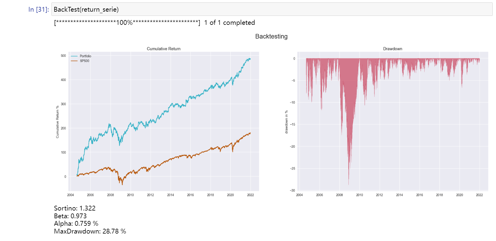
  print(f"MaxDrawdown: {np.round(max_drawdown, 3)} %")